Quickstart to AutoPDEx
In this example, let’s do a finite element analysis of a hyperelastic mechanical punch problem:

Preprocessing
First, we do some imports and activate the double precision, since JAX is using single precsion by default.
[1]:
import jax
from jax import config
import jax.numpy as jnp
import flax
import pygmsh
import meshio
import pyvista as pv

from autopdex import seeder, geometry, solver, utility, models, spaces

config.update("jax_enable_x64", True)
Meshing is (currently) not part of autopdex. Here we use pygmsh for the mesh generation. As element order we choose second order quadrilateral elements.
[2]:
element_order = 2
L = 2.
H = 1.
pts = [[0., 0.], [L, 0.], [L, H], [0., H]]
with pygmsh.occ.Geometry() as geom:
    region = geom.add_polygon(pts, mesh_size=0.1)
    geom.set_recombined_surfaces([region.surface])
    mesh = geom.generate_mesh(order=element_order)
Let’s get the relevant information from the mesh and make it to JAX arrays.
[3]:
n_dim = 2
x_nodes = jnp.asarray(mesh.points[:,:n_dim])
n_nodes = x_nodes.shape[0]
elements = jnp.asarray([ v for k, v in mesh.cells_dict.items() if 'quad' in k])[0]
surface_elements = jnp.asarray([ v for k, v in mesh.cells_dict.items() if 'line' in k])[0]
print("Number of elements: ", elements.shape[0])
print("Number of unknowns: ", n_nodes * n_dim)
Number of elements:  241
Number of unknowns:  2050
For Finite Elements, the Dirichlet conditions are usually imposed by direct nodal imposition. Therefore, we first have to find the concerning nodes. The selection of nodes can be done by means of smooth distance functions. For some primitives, the distance function can be found in the geometry module. The module also contains Rvachev-function operations which can be used for constructing user-defined distance functions. Here, we select the nodes that are close to the lines on which we want to impose the Dirichlet boundary conditions.
[4]:
dirichlet_nodes_left = geometry.on_lines(x_nodes, pts[0], pts[3])
dirichlet_nodes_bottom = geometry.on_lines(x_nodes, pts[0], pts[1])
dirichlet_nodes_top = geometry.on_lines(x_nodes, pts[2], pts[3])
For using the nodal imposition of boundary conditions in autopdex, we have to provide it with a mask that defines which degrees of freedoms shall be constrained.
Below, we fix the displacement in x-direction at the left and top and in y-direction at the bottom by settings the concerning entries to True.
[5]:
selection_left = utility.dof_select(dirichlet_nodes_left, jnp.asarray([True, False]))
selection_bottom = utility.dof_select(dirichlet_nodes_bottom, jnp.asarray([False, True]))
selection_top = utility.dof_select(dirichlet_nodes_top, jnp.asarray([True, False]))
dirichlet_dofs = selection_left + selection_bottom + selection_top
Also, we have to provide the values of the Dirichlet conditions at the Dirichlet nodes. Here: homogeneous Dirichlet conditions.
[6]:
dirichlet_conditions = jnp.zeros_like(dirichlet_dofs, dtype=jnp.float64)
For the imposition of the line load, we can use surface elements. First, the line elements for the Neumann boundary conditions are selected.
[7]:
neumann_selection = geometry.select_elements_on_line(x_nodes, surface_elements, [0, H], [L/2, H])
neumann_elements= surface_elements[neumann_selection]
Now, we have to specify, how the element residual and tangent vectors shall be computed. Isoparametric domain elements based on a weak form are already contained in the models module, but we need to specify the solution space (spaces.fem_iso_line_quad_brick), the integration point positions and weights (Gauß-Legendre) and the weak form. The weak form for a hyperelastic mechanical steady state problem can also be loaded from the models (basically just \(\frac{\partial \psi}{\partial \mathbf{F}} : \delta \mathbf{F}\), with the strain energy function \(\psi\) and the deformation gradient \(\mathbf{F}\)).
[8]:
# Young's modulus and Poisson ratio
youngs_mod_fun = lambda x: 240.5
poisson_ratio = 0.3
poisson_ratio_fun = lambda x, settings: settings['poisson ratio']       # Here we take the Poisson ratio from the settings (and introduce the keyword 'poisson ratio')
                                                                        # in order to be able to take the derivative with respect to the Poisson ratio later on

# Weak form with neo-Hookean strain energy function
weak_form_fun_1 = models.hyperelastic_steady_state_weak(
    models.neo_hooke, youngs_mod_fun, poisson_ratio_fun, 'plain strain')

# isoparametric Q2 elements with fourth order accurate Gauss integration
user_elem_1 = models.isoparametric_domain_element_galerkin(
    weak_form_fun_1,
    spaces.fem_iso_line_quad_brick,
    *seeder.gauss_legendre_nd(dimension = 2, order = 2 * element_order))
Similarly, we can set-up the weak form contribution of the surface load (\(- \mathbf{T} \cdot \delta \mathbf{u}\) with the traction \(\mathbf{T}\)). In order to be able to impose the traction in load steps, we have to multiply the load with the load multiplier.
[9]:
q_0 = -8.0e+2
traction_fun = lambda x, settings: jnp.asarray([0., settings['load multiplier'] * q_0])
weak_form_fun_2 = models.neumann_weak(traction_fun)
user_elem_2 = models.isoparametric_surface_element_galerkin(weak_form_fun_2,
                                                        spaces.fem_iso_line_quad_brick,
                                                        *seeder.gauss_legendre_nd(dimension = 1, order = 2 * element_order),
                                                        tangent_contributions=False)
Finally, we have defined the boundary value problem and have to put it in a form suitable for autopdex to proceed, i.e. the dictionaries static_settings and settings.
[10]:
n_fields = 2
static_settings = flax.core.FrozenDict({
  'number of fields': (n_fields, n_fields),                 # In the tuples, we provide the information for the two domains, the volume and surface integral
  'assembling mode': ('user element', 'user element'),
  'solution structure': ('nodal imposition', 'nodal imposition'),
  'model': (user_elem_1, user_elem_2),
  'solver type': 'newton',
  'solver backend': 'scipy',      # One could also use 'pardiso' (if installed) which is usually faster
  'solver': 'lapack',             # 'lu' in case of 'pardiso'
  'verbose': 1,
})

settings = {
  'dirichlet dofs': dirichlet_dofs,
  'connectivity': (elements, neumann_elements),
  'load multiplier': 0.,
  'poisson ratio': poisson_ratio,
  'node coordinates': x_nodes,
  'dirichlet conditions': dirichlet_conditions,
}
Analysis
Compile and run the adaptive load stepping.
[11]:
dofs_0 = jnp.zeros((n_nodes, n_fields)) # Initial guess for the degrees of freedom
dofs = solver.adaptive_load_stepping(dofs_0, settings, static_settings)[0]
Multiplier: 0.2
Residual after Newton iteration 1: 30.123826347679017
Residual after Newton iteration 2: 7.484234761117104
Residual after Newton iteration 3: 0.8521793502481699
Residual after Newton iteration 4: 0.010471309029161694
Residual after Newton iteration 5: 1.8311066124705274e-06
Residual after Newton iteration 6: 9.895702171411871e-13

Multiplier: 0.4142857142857143
Residual after Newton iteration 1: 26.044600550086802
Residual after Newton iteration 2: 6.552331902728065
Residual after Newton iteration 3: 0.9245626445289336
Residual after Newton iteration 4: 0.03481961828160253
Residual after Newton iteration 5: 5.320097873054512e-05
Residual after Newton iteration 6: 1.2811750584041405e-10
Residual after Newton iteration 7: 2.9816550509507755e-12

Multiplier: 0.6285714285714286
Residual after Newton iteration 1: 21.84487496054895
Residual after Newton iteration 2: 3.030257385932747
Residual after Newton iteration 3: 0.17124924912790535
Residual after Newton iteration 4: 0.0012620383197380464
Residual after Newton iteration 5: 6.663511400719465e-08
Residual after Newton iteration 6: 6.324077425210025e-12

Multiplier: 0.8581632653061224
Residual after Newton iteration 1: 26.20471352427922
Residual after Newton iteration 2: 3.187869256332422
Residual after Newton iteration 3: 0.05592446538434068
Residual after Newton iteration 4: 4.42660610828264e-05
Residual after Newton iteration 5: 5.367347021062305e-11

Multiplier: 1.0
Residual after Newton iteration 1: 7.735572126180451
Residual after Newton iteration 2: 0.2883951631987405
Residual after Newton iteration 3: 0.0005834065396459414
Residual after Newton iteration 4: 2.5652515233467498e-09
Residual after Newton iteration 5: 2.1216160148900787e-11
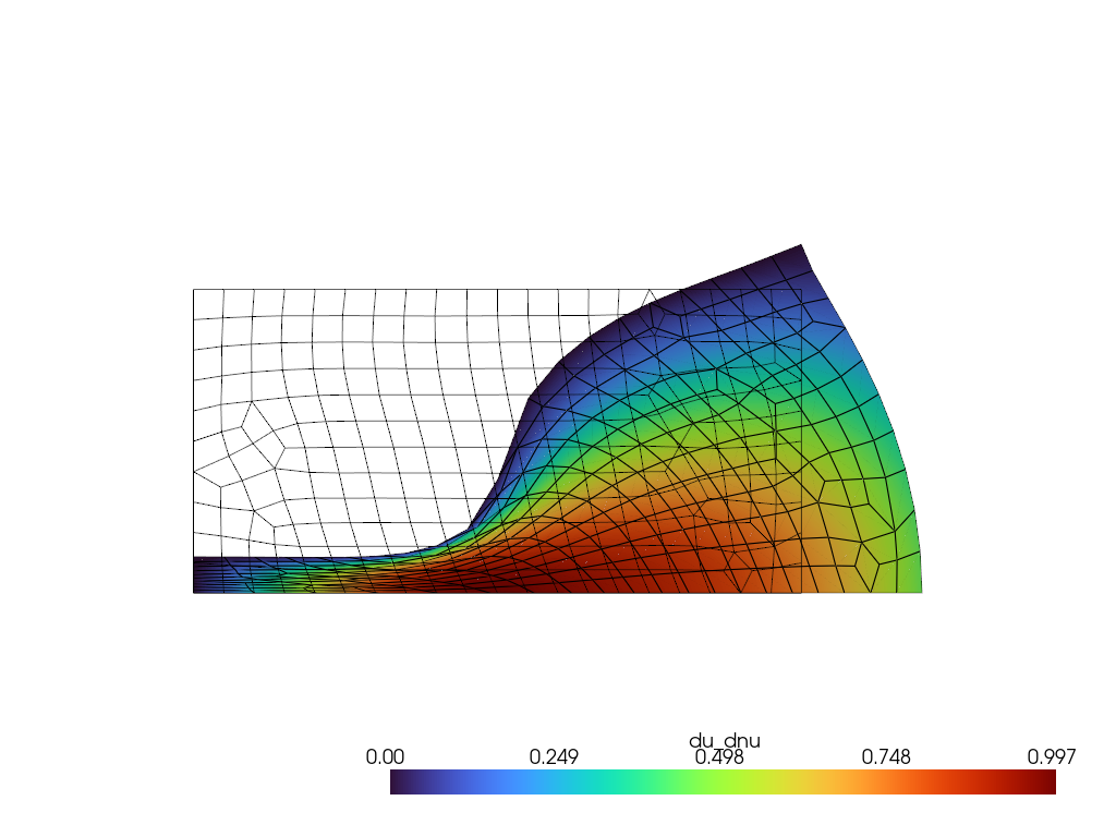
The adaptive_load_stepping function is automatically made differentiable with respect to the settings by specifying the differentiation mode. Here, we exemplarily compute the derivative of the degrees of freedom with respect to the Poisson ratio. For taking derivatives of many values (dofs) with respect to a few variables (poisson ratio), the forward mode performs best.
[12]:
static_settings = static_settings.copy({'verbose': -1})
@jax.jit
def diffable_solve(poisson_ratio, settings):
    settings['poisson ratio'] = poisson_ratio
    return solver.adaptive_load_stepping(dofs_0, settings, static_settings, path_dependent=False, implicit_diff_mode='forward')[0]
compute_sensitivities = jax.jit(jax.jacfwd(diffable_solve))
du_dnu = compute_sensitivities(poisson_ratio, settings)
In the first call, it is compiled. Subsequent calls are faster
[13]:
%timeit -r 1 -n 1 diffable_solve(poisson_ratio, settings).block_until_ready()
4.18 s ± 0 ns per loop (mean ± std. dev. of 1 run, 1 loop each)
[14]:
%timeit diffable_solve(poisson_ratio, settings).block_until_ready()
640 ms ± 86.3 ms per loop (mean ± std. dev. of 7 runs, 1 loop each)
Computing the sensitivity takes in this case only marginally longer
[15]:
%timeit compute_sensitivities(poisson_ratio, settings).block_until_ready()
657 ms ± 74.6 ms per loop (mean ± std. dev. of 7 runs, 1 loop each)
Postprocessing
Export as .vtk for Paraview
[16]:
points = mesh.points
cells = jnp.asarray([ v for k, v in mesh.cells_dict.items() if 'quad' in k])[0]
mesh = meshio.Mesh(
    points,
    {'quad': cells[:,:4]},
    point_data={
        "u": jnp.pad(dofs, ((0, 0), (0, 1)), constant_values=0),
        "du_dnu": jnp.pad(du_dnu, ((0, 0), (0, 1)), constant_values=0),
    },
)
mesh.write("./punch_test.vtk")
Visualization with pyvista
[17]:
pv.set_jupyter_backend('static')
plotter = pv.Plotter()
pv_mesh = pv.read("./punch_test.vtk")
warped_mesh = pv_mesh.warp_by_vector('u')
plotter.add_mesh(warped_mesh, scalars='du_dnu', component=0, show_edges=True, cmap='turbo')
plotter.add_mesh(pv_mesh, style='wireframe', color='black')
plotter.view_xy()
plotter.show()