Examplary input files

Here is a list of examples demonstrating the functionality of AutoPDEx.

Example 1: Cook’s membrane (Quadrilaterals in Hyperelasticity)

Link: quadrilaterals_autopdex_and_acegen.py

This example demonstrates the solution of Cook’s membrane problem using custom elements from the autopdex.models library and an exemplary external AceGen-generated C routine.

The main steps include:

1. Definition of geometry and boundary conditions.

2. Mesh generation using pygmsh and conversion to JAX arrays.

3. Selection of nodes for boundary conditions and setup of Dirichlet conditions.

4. Definition of material properties for the neo-Hookean model.

5. Optional use of an AceGen-generated shared library for custom element computation.

6. Element definition for hyperelastic steady-state weak form.

7. Element definition for imposition of Neumann boundary conditions.

8. Solver settings and configuration using flax.core.FrozenDict.

9. Adaptive load stepping solver for nonlinear analysis.

10. Export results in VTK format for ParaView.

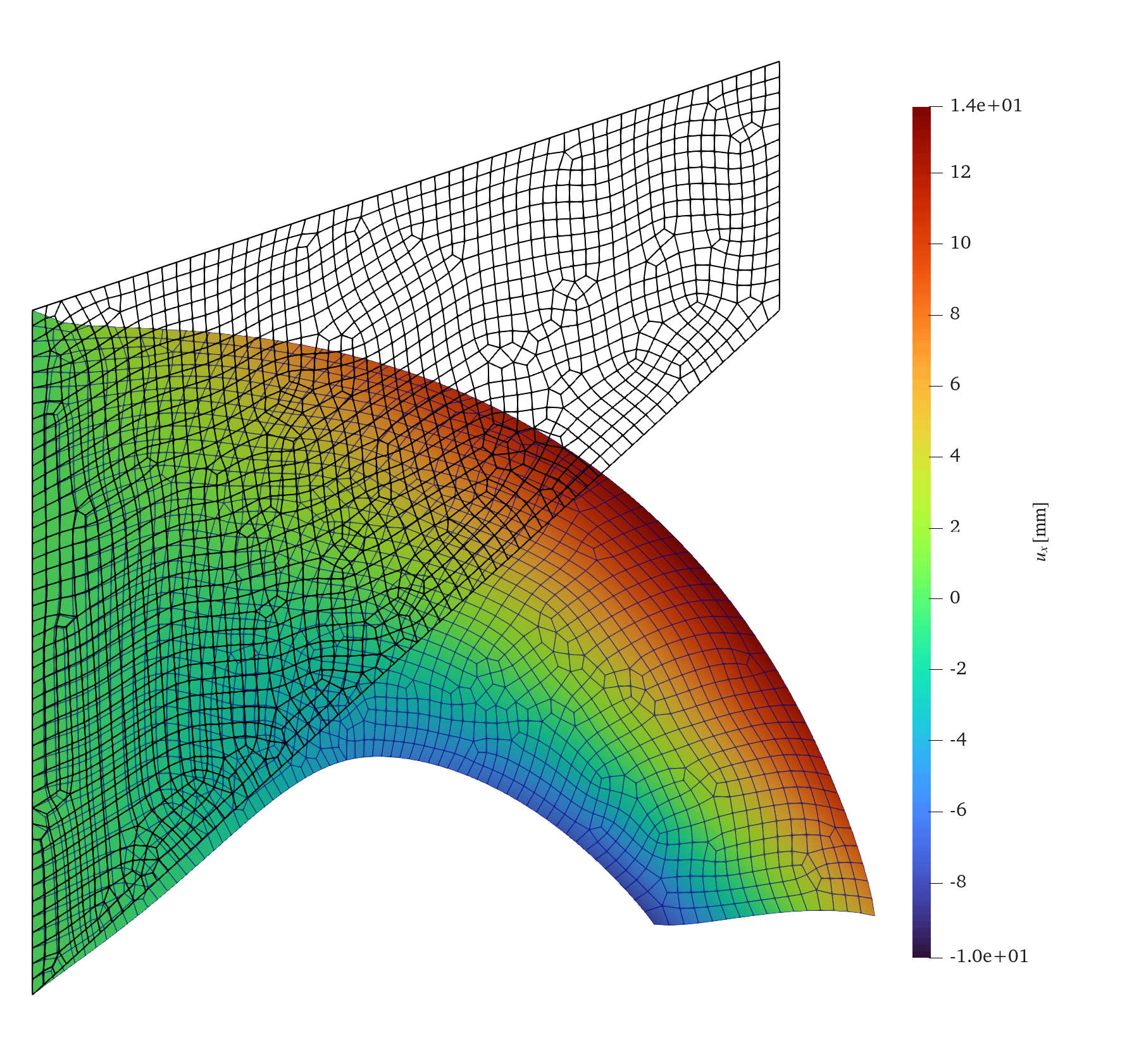
Figure: Here is a picture generated with ParaView from the output file of the above code that shows the initial configuration as a wireframe and the deformed configuration with colored horizontal displacements.

Further examples, based on the Cook’s membrane include:

• triangles_h_refinement.py: Simplex-shaped elements based on least squares, integrated in the initial configuration.

• non-homogeneous_dirichlet_conditions.py: Nodal imposition of non-homogeneous Dirichlet conditions.

• quadrilaterals_p_refinement.py: A p-refinement with isoparametric quadrilateral elements.

• least_square_fem_rvachev_structure.py: First order system least square Finite Elements as a Rvachev solution structure.

• moving_least_squares_least_square_fos.py: Moving Least Square solution structure based on a first order system.

Example 2: Transient heat conduction (forward- and backward-Euler)

Link: maze_forward_euler.py

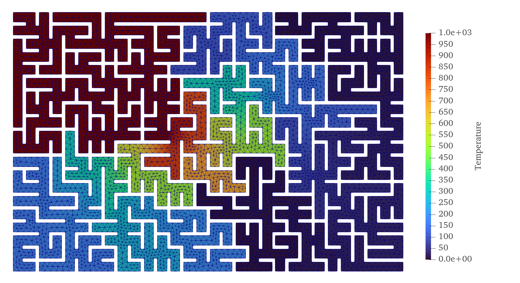
The example demonstrates how to implement an explicit time integration of the transient heat conduction equation in AutoPDEx. Three domains are introduced. The first domain includes the virtual work of the internal driving forces or the weak form of the Laplace equation. The second domain covers the surface integral over the Neumann boundary (an edge of the maze in the upper left area). The third domain encompasses the transient term (forward Euler), integrated by collocation. The resulting system of equations for a time step is diagonal and can be efficiently solved locally. An analogous version with backward Euler, which is not subject to the Courant-Friedrichs-Lewy time step restriction, can be found in the example maze_backward_euler.py.

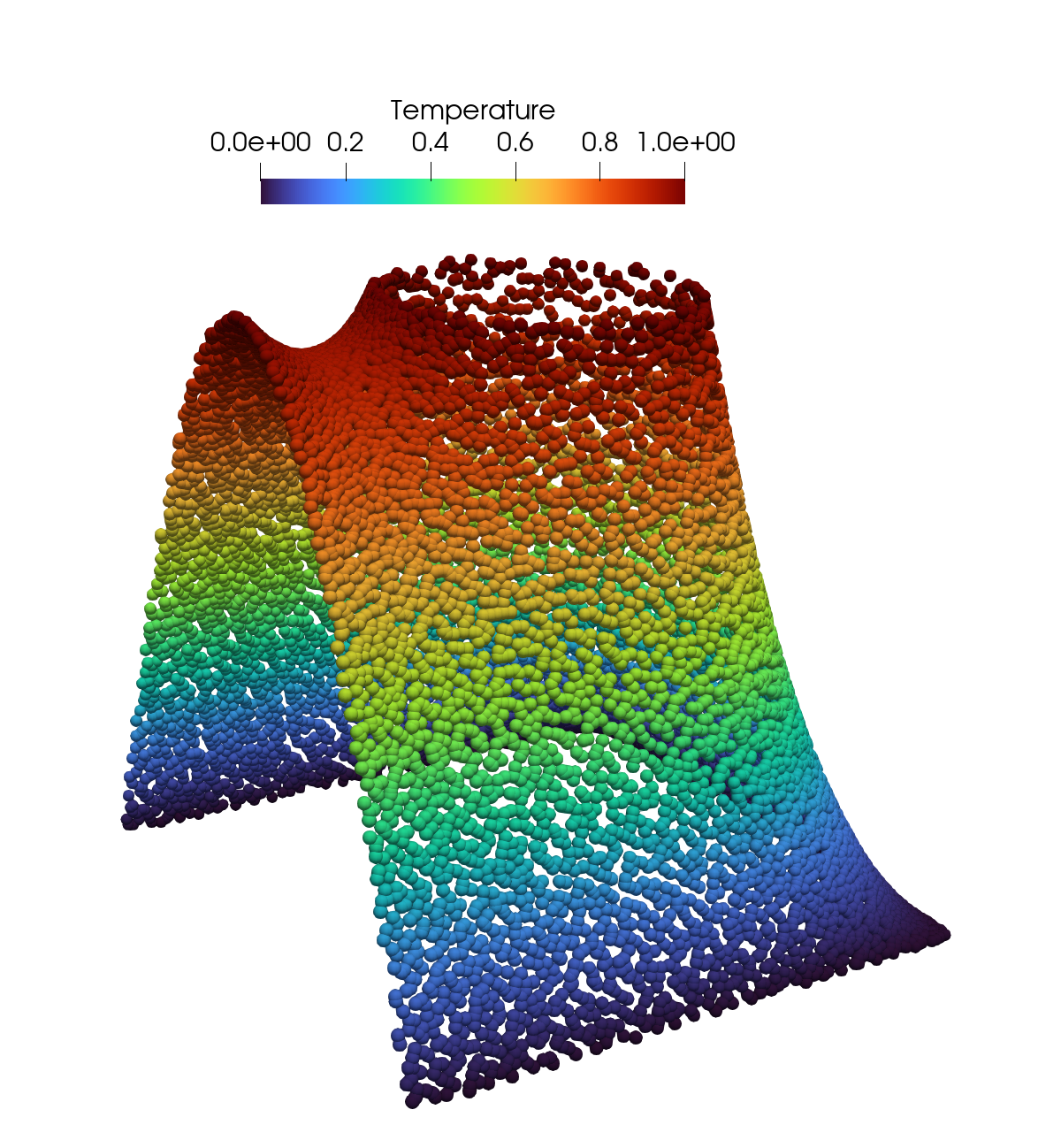
Figure: The image shows a snapshot of the temperature distribution within the maze visualized with ParaView

Further examples related to transient heat transfer:

• maze_backward_euler.py: Same as above, but with implicit backward Euler time discretization.

• space_time_fos_dirichlet_neumann_robin.py: Space-time solution of transient heat conduction as first order system with combined Dirichlet, Neumann and Robin conditions.

• space_time_different_solvers.py: Comparison of different solver backends.

Example 3: Wave equation (least square method of first order system)

Link: wave_equation.py

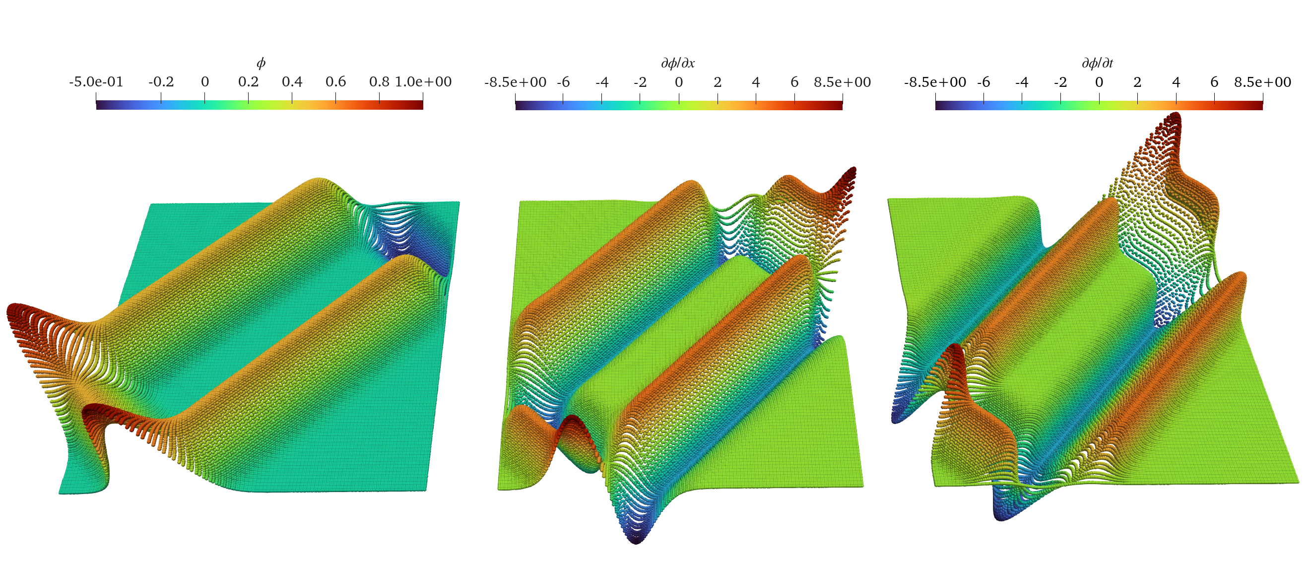
In this example, the wave equation is solved on the square domain \((x, t)\) with \(x \in (0, 1)\) and \(t \in (0, 1)\). The problem is formulated as a first-order system, and the solution is searched using a least-squares variational method. For the solution space, meshfree moving least squares (MLS) shape functions of second order are used, with integration performed on a background grid (as in the Element-Free Galerkin (EFG) method) using Gaussian quadrature. The application of boundary conditions is achieved through the solution structure for first-order systems using Rvachev distance functions to the respective boundary segments.

Figure: The gauss-point quantities for the field (left), its spatial derivative (middle) and its temporal rate (right) are depicted. One can clearly see the effects of wave propagation, superposition and reflection at the free and clamped end.

Example 4: Steady-state Navier-Stokes equations (adaptive load stepping and nonlinear minimization)

Link: circle_in_channel.py

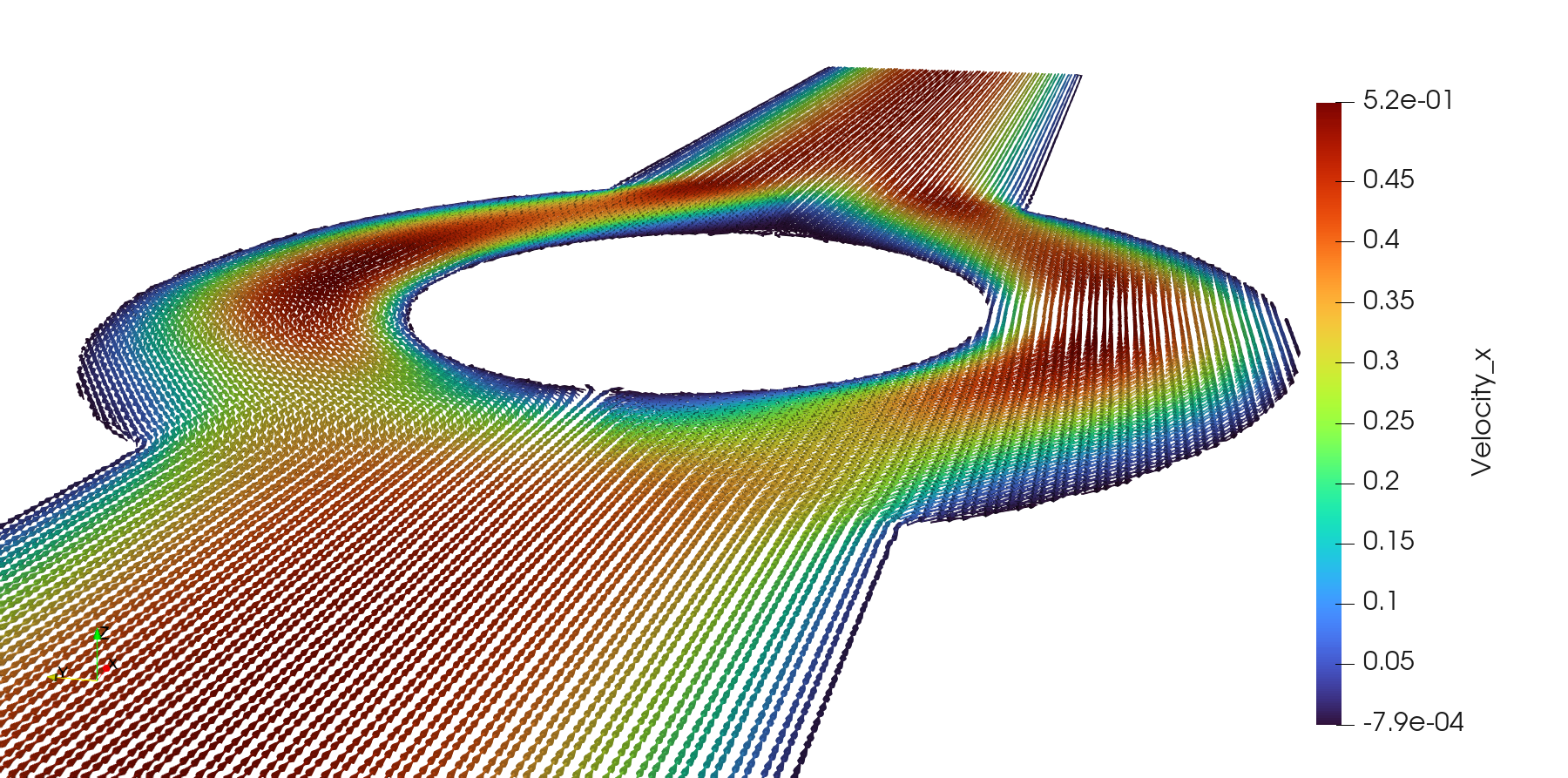
For this example, the model problem described in nvidia/modulus/examples/annular_ring is used. The stationary Navier-Stokes equations are treated here using a Galerkin method in the strong form or a least-squares method. A moving least squares solution structure is used as the solution space. The nonlinear equations are solved by incrementally increasing the inlet velocity using the Newton-Raphson method. Alternatively, for the least squares variational method, a nonlinear minimizer such as the Limited Memory Broyden–Fletcher–Goldfarb–Shanno (L-BFGS) algorithm can be applied.

Figure: Steady-state flow field of a Moving Least Squares Galerkin solution.

Related examples:

• lid_driven_cavity.py: Comparison of Galerkin and least square variational schemes.

Example 5: Implicit differentiation (uncertainty estimation)

Link: uncertainty_estimation_hyperelastic.py

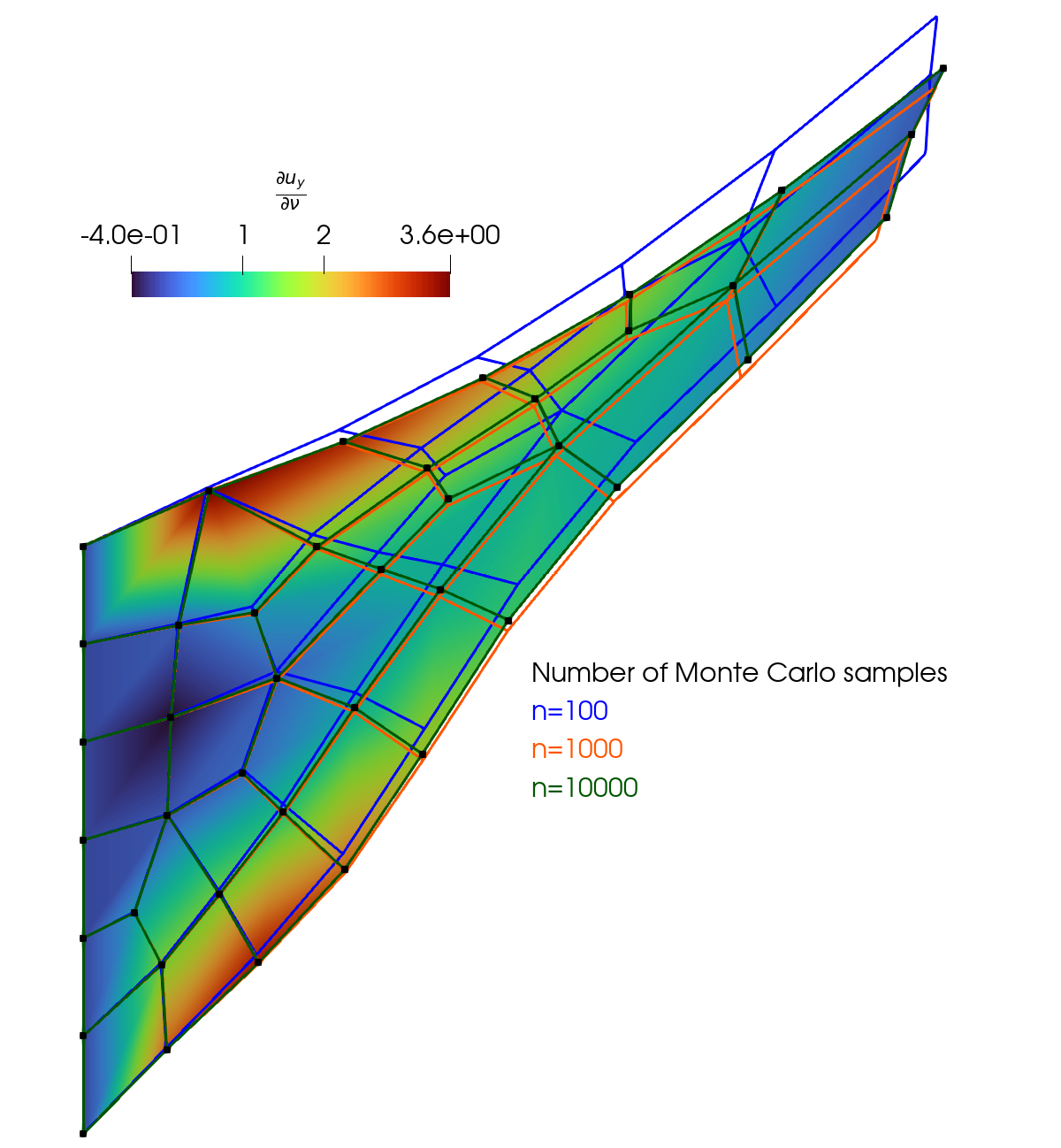
This example addresses Cook’s membrane problem where the Young’s modulus and Poisson’s ratio follow a multivariate normal distribution. The goal is to compute the expectation and standard deviation of the displacement field. Two approaches are compared: the Monte Carlo method and an approach based on a Taylor series expansion. For the Taylor series expansion, the derivatives of the displacement degrees of freedom with respect to Young’s modulus and Poisson’s ratio are required. These sensitivities are calculated using automatic implicit differentiation based on the implicit function theorem.

Figure: The three wireframes represent the scaled standard deviation of the displacement field for three Monte Carlo simulations. With 10,000 samples, the Monte Carlo solution aligns visually with the black nodes of the solution calculated using the Taylor expansion. The coloring represents the sensitivity of the vertical displacement field with respect to Poisson’s ratio.

Example 6: Further examples

List of further examples:

• mls_rfm.py: Dirichlet problem of the Laplace equation in 2d: [0,1]x[0,1] with cutout circle (midpoint=[0.5,0.5], radius=0.25). Demonstration of quasi-random sampling in regions defined by signed distance functions.

• pinn_rfm.py: Neural network as user-defined solution space, boundary conditions through R functions.

• fos_coupled_neumann_boundary.py: First order least square system of Laplace equation with coupled Neumann boundary conditions on circular cutout.

• poisson.py: Demonstration of compile time reduction by manually pre-compiling solution structures.

• transport.py: Transport equation as moving least square solution structure with least square variational method.

• burgers_equation.py: Solution of the Burgers equation using moving least squares.

• geometry_examples.py: Interactive visualization of smooth distance functions.

Figure: Exemplary result of solving the Laplace equation with a Moving Least Square solution structure on a square-shaped domain with cutout (mls_rfm.py).